CFD Codes in Python
In my 6th semster, I have taken up the elective course under Dr. Yogesh G Bhumkar, Associate Professor, School of Mechanical Sciences. I was introduced to Python for developing inhouse codes to the problems. Python plays a pivotal role in Computational Fluid Dynamics (CFD), offering versatile libraries like OpenFOAM, PyTorch, and NumPy. It enables efficient simulation, data manipulation, and visualization, accelerating CFD research and analysis. Python's simplicity and extensibility make it an essential tool for engineers and researchers in the field. Prior to this I was used in doing simulations in ANSYS, where I used commercial CFD codes to solve the problems. Some of the problems I have worked on, are Dirichlet Problem, Neumann Problem, Poisson Equation, and solving Laplacian Heat Equation in different scenarios. The setup for the first three problem scenarios is as follows:
A 2 dimensional square plate is considered as the grid for our understanding. Temperature applied on the ends, change according to the boundary conditions set by us.
import numpy as np
import matplotlib.pyplot as plt

l = 10.0
b = 10.0
N = 41
dx = l / (N - 1)
dy = b / (N - 1)

x = np.zeros((N, N))
y = np.zeros((N, N))

for i in range(N):
	for j in range(N):
		x[i, j] = dx * j
		y[i, j] = dy * i

T = np.ones((N, N))
T[0, :] = 100
T[:, 0] = 50
T[N - 1, :] = 75
T[:, N - 1] = 50

A = 2 / (dx ** 2) + 2 / (dy ** 2)

for ct in range(1000):
	for j in range(1, N - 1):
		for i in range(1, N - 1):
			T[i, j] = (((T[i + 1, j] + T[i - 1, j]) / (dx ** 2))+ ((T[i, j + 1] + T[i, j - 1]) / (dy ** 2))) / A

plt.contourf(x, y, T, levels=20, cmap='rainbow')
plt.colorbar(label='Temperature')
plt.xlabel('X')
plt.ylabel('Y')
plt.title('Temperature Contour')
plt.show()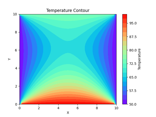
import numpy as np
import matplotlib.pyplot as plt

l = 10.0
b = 10.0
N = 11
dx = l / (N - 1)
dy = b / (N - 1)

# Discretization of domain
x = np.zeros((N, N))
y = np.zeros((N, N))
for i in range(N):
	for j in range(N):
		x[i, j] = dx * (j)
		y[i, j] = dy * (i)

# Boundary condition
T = np.ones((N, N))
T[:, 0] = 100
T[:, -1] = 50

# Iterative solving of PDE
for ct in range(10000):
	for j in range(1, N - 1):
		for i in range(1, N - 1):
			T[i, j] = (T[i + 1, j] + T[i - 1, j] + T[i, j + 1] + T[i, j - 1]) / 4
	T[0, 1:N - 1] = T[1, 1:N - 1]
	T[N - 1, 1:N - 1] = T[N - 2, 1:N - 1]

# Plot the contour
plt.contourf(x, y, T, cmap='hot')
plt.colorbar(label='Temperature')
plt.xlabel('X')
plt.ylabel('Y')
plt.title('Temperature Contour')
plt.show()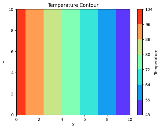
import numpy as np
import matplotlib.pyplot as plt

l = 10.0
b = 10.0
N = 41
dx = l / (N - 1)
dy = b / (N - 1)

# Discretization of domain
x = np.zeros((N, N))
y = np.zeros((N, N))
for i in range(N):
	for j in range(N):
		x[i, j] = dx * (j)
		y[i, j] = dy * (i)

# Boundary condition
T = np.ones((N, N))

# Iterative solution of PDE
A = (2 / (dx**2)) + (2 / (dy**2))
for ct in range(10000):
	for j in range(1, N - 1):
		for i in range(1, N - 1):
			T[i, j] = (((T[i + 1, j] + T[i - 1, j]) / (dx**2)) + ((T[i, j + 1] + T[i, j - 1]) / (dy**2))) / A + \ (100 / A) * np.exp(-8 * ((x[i, j] - 5)**2 + (y[i, j] - 5)**2))

# Plot the contour
plt.contourf(x, y, T, cmap='rainbow')
plt.colorbar()
plt.xlabel('x')
plt.ylabel('y')
plt.title('Temperature Distribution')
plt.show()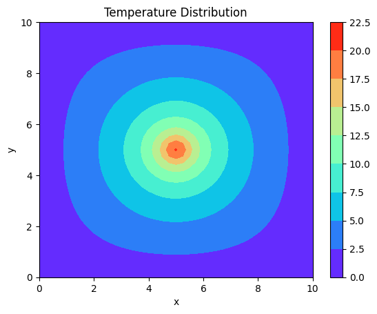
Here, represents the rate of change of temperature with respect to time, α is the thermal diffusivity, and ∇²u represents the Laplacian of temperature. This equation models the time-dependent heat conduction in a rod. The initial conditions are the temperature being 25°. The other details can be found in the code:
import numpy as np
import matplotlib.pyplot as plt

x = np.arange(1, 101)  # Domain definition
T = np.zeros((1000, 100))  # Initialization as an array

# Initializing the first time step using the given formula
T[0, :] = 75 * np.exp(-0.009 * ((x - 50) ** 2)) + 25

# Defining Timestep (dt), Cell size(dx), PDE parameter (alpha)
a = 0.1
dt = 1
dx = 1

# Solving Parabolic PDE
for t in range(1, 1000):
	for i in range(1, 99):
		T[t, 0] = 25
		T[t, 99] = 25
		T[t, i] = T[t - 1, i] + (a * dx / (dt ** 2)) * (T[t - 1, i + 1] - 2 * T[t - 1, i] + T[t - 1, i - 1])

# Visualizing over every 100 timesteps
for k in range(0, 1000, 100):
	time_in_seconds = k * dt
	plt.plot(x, T[k, :], label=f'Time: {time_in_seconds:.0f} s')

plt.xlabel('x')
plt.ylabel('Temperature (T)')
plt.title('Temperature Evolution over Time')
plt.legend()  # Place the legend in the upper right corner
plt.show()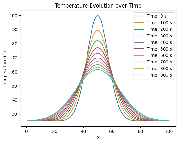
import numpy as np
import matplotlib.pyplot as plt

x = np.arange(1, 101)  # Domain definition
y = np.concatenate((np.zeros(30), np.arange(0, np.pi + np.pi / 31, np.pi / 31), np.zeros(38)))
u = np.zeros((10, 100))  # Initialization as an array

# Initializing the first time step using sine of y
u[0, :] = np.sin(y)
a = 0.1
dt = 1
dx = 1
c = -1

for t in range(1, 10):
	for i in range(1, 99):
		u[t, i] = u[t - 1, i] - 0.5 * ((c * dt) / dx) * (u[t - 1, i + 1] - u[t - 1, i - 1])

# Visualizing over each time step
for k in range(10):
	time_step = k + 1
	plt.plot(x, u[k, :], label=f'Time Step {time_step}', linestyle='-', linewidth=1)

plt.title('Hyperbolic Wave Equation', fontweight='bold')
plt.xlabel('1D Spatial Domain', fontweight='bold')
plt.ylabel('Amplitude', fontweight='bold')
plt.show()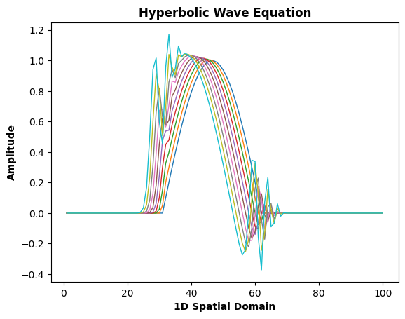
In the first case, our consideration is directed towards openings strategically situated diagonally opposite to each other, maintaining a mutually facing alignment. This particular arrangement is mirrored by the observable pattern of streamlines. The code is as follows:
import numpy as np
import matplotlib.pyplot as plt

l = 10.0
b = 10.0
N = 41
dx = l / (N - 1)
dy = b / (N - 1)

# Discretisation of domain
x = np.zeros((N, N))
y = np.zeros((N, N))
for i in range(N):
	for j in range(N):
		x[i, j] = dx * j
		y[i, j] = dy * i

# Boundary condition
p = np.ones((N, N))
p[:, 0] = 2
p[N - 1, 0:33] = 2
p[0, 8:N] = 4
p[:, N - 1] = 4
p[0, 0:9] = np.arange(2, 4.25, 0.25)
p[N - 1, 32:N] = np.arange(2, 4.25, 0.25)

A = 2 / dx ** 2 + 2 / dy ** 2

# Solution of PDE
for ct in range(10000):
	for i in range(1, N - 1):
		for j in range(1, N - 1):
			p[i, j] = ((p[i + 1, j] + p[i - 1, j]) / dx ** 2 + (p[i, j + 1] + p[i, j - 1]) / dy ** 2) / A

# Plotting rainbow-filled contours and contour lines
plt.contourf(x, y, np.rot90(p, 2), 50, cmap='rainbow')
contour_lines = plt.contour(x, y, np.rot90(p, 2), 15, colors='black')
plt.clabel(contour_lines, inline=True, fontsize=8)
plt.xlabel('X')
plt.ylabel('Y')
plt.title('Rainbow-Filled Contours with Contour Lines')
plt.colorbar(label='Value')
plt.show()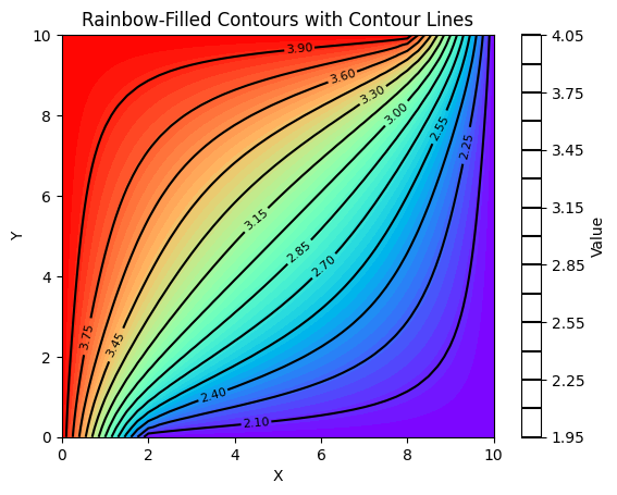
import numpy as np
import matplotlib.pyplot as plt

l = 10.0
b = 10.0
N = 41
dx = l / (N - 1)
dy = b / (N - 1)

# Discretisation of domain
x = np.zeros((N, N))
y = np.zeros((N, N))
for i in range(N):
	for j in range(N):
		x[i, j] = dx * j
		y[i, j] = dy * i

# Boundary condition
p = np.ones((N, N))

p[:, 0] = 2
p[40, 0:7] = 2
p[40,7:12] = np.arange(2 + 1/6, 2 + 5/6, 1/6)
p[40,11:18] = 8/3
p[40,18:23] = np.arange(8/3 + 1/6, 8/3 + 5/6, 1/6)
p[40,22:29] = 10/3
p[40,29:34] = np.arange(10/3 + 1/6, 10/3 + 5/6, 1/6)
p[40,33:40] = 4
p[0, 0:8] = np.arange(2, 3.75 + 0.25, 0.25)
p[0, 8:40] = 4
p[:, 40] = 4

A = 2 / dx ** 2 + 2 / dy ** 2

# Solution of PDE
for ct in range(10000):
	for i in range(1, N - 1):
		for j in range(1, N - 1):
			p[i, j] = ((p[i + 1, j] + p[i - 1, j]) / dx ** 2 + (p[i, j + 1] + p[i, j - 1]) / dy ** 2) / A

# Streamline visualization using contours

plt.contourf(x, y, np.rot90(p, 2), 50, cmap='rainbow')
contour_lines = plt.contour(x, y, np.rot90(p, 2), 30, colors='black')
plt.clabel(contour_lines, inline=True, fontsize=8)
plt.xlabel('X')
plt.ylabel('Y')
plt.title('Rainbow-Filled Contours with Contour Lines')
plt.colorbar(label='Value')
plt.show()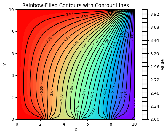
I would like to thank Dr. Yogesh G Bhumkar for his guidance and constant encouragement towards taking up the challenge to develop the codes instead of using the available commercial codes. His interactive classroom approach has inspired me to venture into this new field. I would like to take this opportunity to thank my batchmate, Mr. Bharath Ram for helping me out in clutch situations.

